ECE298-S19
Linear complex algebra: ECE Webpage ECE298-F19; ECE-298-F19; UIUC Course Explorer: ECE-298-F19; Time: TBD MWF; Location: TBD ECEB (official); Register
- Professor: Jont B. Allen (jontalle@illinois.edu), TA: TBD
- Syllabus: ECE298-F19; *Exams: Exam I; Exam II; About the final; Grades:*Office Hours: Thur TBD Location: TBD ECEB Mathematical notation by topic, alpha-order, use of Functions and their History, Mathematical vignettes.
- Tools: Matlab, Octave, Latex
- This week's schedule
ECE 298JA Schedule (Fall 2019)
| L | W | D | Date | Lecture and Assignment |
| Part I: Number systems (10 Lectures) | ||||
| 1 | 1 | M | 8/28 | Introduction & Historical Overview; Lecture 0: pdf;
The Pythagorean Theorem & the Three streams: 1) Number systems (Integers, rationals) 2) Geometry 3) {$\infty$} {$\rightarrow$} Set theory {$\rightarrow$} Calculus symbols |
| 2 | W | 9/1 | Lecture: The role of physics in Mathematics, Eigen analysis; The Fundamental theorems of Mathematics: Read: Class-notes | |
| 3 | F | 9/18 | Lecture: Analytic geometry as physics (Stream 2) Polynomials, Analytic functions, {$\infty$} Series Taylor series; ROC; expansion point Read: Class-notes Homework 1 (NS-1): Basic Matlab commands: pdf (v. 1.06), Due 9/6 (1 week); help | |
| 4 | M | 9/22 | Lecture: Polynomial root classification by convolution; Summarize Lec 3: Series representations of analytic functions, ROC Historical notes on complex numbers: Solution of the quadratic (Brahmagupta, 628), cubic (c1545), quartic (c1535), quintic cannot be solved (Abel, 1826) and much more Fundamental Thm of Algebra (pdf) & Read: Class-notes | |
| 5 | 2 | W | 9/25 | Lecture: Residue expansions of rational functions, Impedance {$Z(s) = \frac{P_m(s)}{P_n(s)}$} and its utility in Engineering applications Read: Class-notes |
| 6 | F | 9/27 | Lecture: Analytic Geometry; Scalar and vector products Read: Class-notes NS-1 Due Homework 2 (AE-1) Polynomials & Analytic functions and their inverse, Convolution, Newton's method (pdf, 1 week) | |
| 7 | M | 9/29 | Lecture: Gaussian elimination (intersection); Pivot matrices {$(\Pi_n)$}: {$U = \Pi_n^N P_n A$} gives upper-diagional {$U$} Read: Class-notes | |
| 8 | 6 | W | 10/2 | Lecture: Transmission matrix method (composition of polynomials, bilinear transformation) Read: Class-notes |
| 9 | F | 10/4 | Lecture: The Riemann sphere (1851); (the extended plane) pdf Mobius Transformation (youtube, HiRes), pdf description Mobius composition transformations, as matrices Software: Octave: zviz.zip, python Read: Class-notes AE-1 due Homework 3 (AE-2): Linear systems of equations; Gaussian elimination; ABCD method; (pdf Due 1 week) | |
| 10 | M | 10/6 | Lecture: Visualizing complex valued functions Colorized plots of rational functions
Read: Class-notes | |
| 11 | 7 | W | 10/9 | Lecture:Read: Class-notes Fourier Transforms (signals) Fourier Transform (wikipedia), Notes on the Fourier series and transform from ECE 310 (including tables of transforms and derivations of transform properties) |
| 12 | F | 10/11 | Lecture: AE-2 Due Laplace transforms (systems); The importance of Causality Convolution of the step function: {$u(t) \leftrightarrow 1/s$} vs. {$2\tilde{u}(t) \equiv 1+ \mbox{sgn}(t) \leftrightarrow 2\pi \delta(\omega) + 2/j\omega$}
| |
| 13 | M | 10/13 | Lecture:Read: Class-notes; Laplace Transform, Types of Fourier transforms The 10 postulates of Systems (aka, Networks) pdf The important role of the Laplace transform re impedance: {$z(t) \leftrightarrow Z(s)$} A.E. Kennelly introduces complex impedance, 1893 pdf Fundamental limits of the Fourier re the Laplace Transform: {$\tilde{u}(t)$} vs. {$u(t)$} | |
| 14 | 8 | W | 10/16 | Lecture: Integration in the complex plane: FTC vs. FTCC Analytic vs complex analytic functions and Taylor formula Calculus of the complex {$s=\sigma+j\omega$} plane: {$dF(s)/ds$}, {$\int F(s) ds$} (Boas, see page 8) The convergent analytic power series: Region of convergence (ROC) Complex-analytic series representations: (1 vs. 2 sided); ROC of {$1/(1-s), 1/(1-x^2), -\ln(1-s)$} 1) Series; 2) Residues; 3) pole-zeros; 4) Analytic properties Euler's standard circular-function package (Logs, exp, sin/cos); Inversion of analytic functions: Example: {$\tan^{-1}(z) = \frac{1}{2i}\ln \frac{i-z}{i+z}$}, the inverse of Euler's formula (1728) Read: Class-notes |
| 15 | F | 10/20 | Lecture:
AE-2 Due | |
| 16 | 9 | M | 10/23 | Lecture: Complex analytic functions and Brune impedance Complex impedance functions {$Z(s)$}, {$\Re Z(\sigma>0) \ge 0$}, Simple poles and zeros & 9 Postulates Time-domain impedance {$z(t) \leftrightarrow Z(s) \Rightarrow v(t) = z(t) \star i(t) $} defines power Read: Class-notes |
| 17 | W | 10/25 | Lecture: Time out: Come with questions: Review session on: multi-valued functions, complex integration, Riemann sheets, colorized plots, branch cuts, Review of Fundamental Theorems of complex analytic functions. Laplace's equation and its role in Engineering Physics. Impedance. What is the difference between a mass and an inductor? Nonlinear elements; Examples of systems and the 10 postulates of systems. | |
| 18 | F | 10/27 | Lecture: Three complex integration Theorems: Part I 1) Cauchy's Integral Theorem: {$\oint f(z) dz =0$} (Boas p. 45) vs. 2D Green's Thm (p. 49); Stokes (Thm, Bio) AE-3 due Homework 5 (DE-1): Series, differentiation, CR conditions, Bi-Harmonic functions: pdf, Due Oct 30 | |
| 19 | 10 44 | M | 10/30 | Lecture: Three complex integration Theorems: Part II 2) Cauchy's Integral Formula: {$\frac{1}{2\pi j} \displaystyle \oint_{{\partial}_{\gamma}} \frac{f(z)}{z-z_0}dz = f(z_0) \, U(\gamma) \equiv 0$} if {$z_0 \notin \gamma^\circ$} 3) Cauchy's Residue Theorem; Example by brute force integration: {$\oint_{|s|=1} \frac{ds}{s}= 2\pi j$} Read: Class-notes & Boas p. 33-43 Complex Integration; Cauchy's Theorem |
| 20 | W | 11/1 | Lecture: The Inverse Laplace Transform (ILT); poles and the Residue expansion: The case for causality {$t<0$} Cauchy's Residue theorem {$\Leftrightarrow$} 2D Green's Thm (in {$\mathbb C$}) Read: Class-notes | |
| 21 | F | 11/3 | Lecture: Inverse Laplace Transform: Use of the Residue theorem {$t>0$} Case for causality: Closing the contour: ROC as a function of {$e^{st}$}. Examples: {$F(s)=1 \leftrightarrow \delta(t)$} and {$u(t) \leftrightarrow 1/s$} Case of RC impedance {$ z(t) = R\delta(t)+u(t)/C \leftrightarrow R+1/sC $} RC admittance {$ y(t) = e^{-t}u(t) \leftrightarrow 1/(s+1) $} Semi-capacitor: {$ u(t)/\sqrt{t} \leftrightarrow \sqrt{\pi/s} $} DE-1 due | |
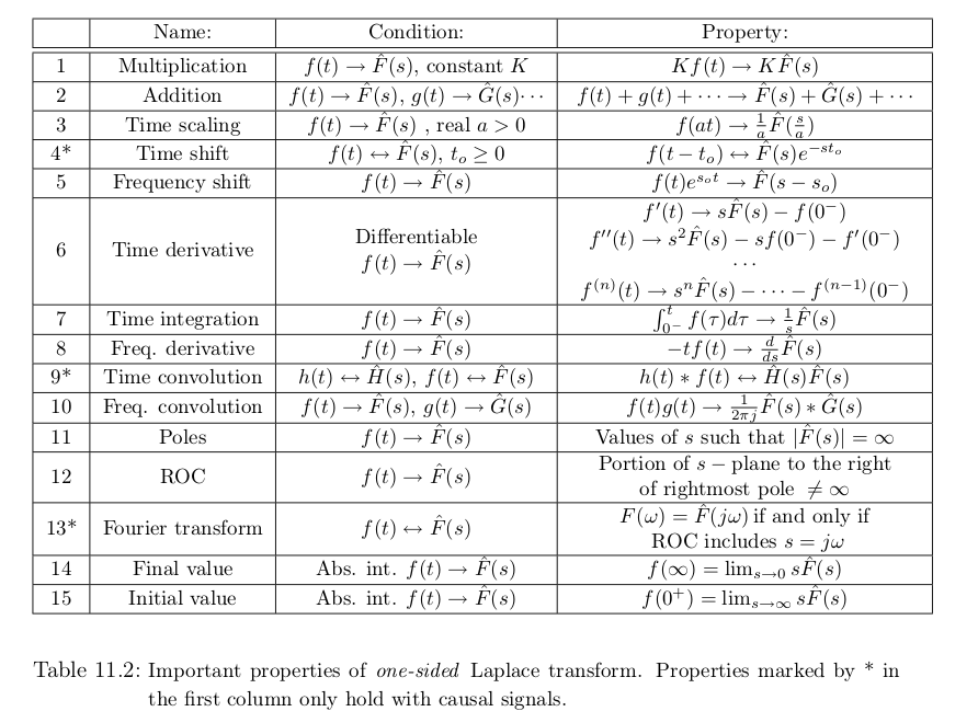
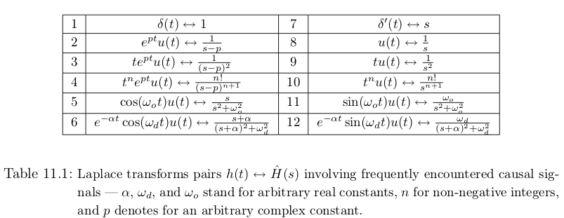
| 22 | 11 45 | M | 11/6 | Lecture: General properties of Laplace Transforms: Modulation, Translation, Convolution, periodic functions, etc. (png) Table of common LT pairs (png) Read: Class-notes |
| 23 | W | 11/8 | Lecture: Review of Laplace Transforms, Integral theorems, etc Sol to DE-3 handout Read: Class-notes | |
| 24 | F | 11/10 | Lecture: General properties of Impedance (Z) and Transmission (ABCD) functions: Impedance {$Z(s) = V(s)/I(s) \rightarrow $} Minimum phase impedance {$\rightarrow$} Simple poles & zeros in LHP ({$\sigma \le 0$}) Transfer {$H(s)=V_2/V_1, I_2/I_1 \rightarrow $} Allpass: {$|e^{-\jmath\phi(\omega)}|=1 \rightarrow$} poles in LHP, zeros in RHP Wiener's factorization theorem: {$H(s) = M(s)A(s)$} with factors Minimum phase {$M(s)$} & Allpass {$A(s)$} Exam II TBD DE-2 Due Homework 7 (DE-3): pdf, Due Nov 10 | |
| 25 | 13 48 | M | 11/27 | Lecture:Read: Class-notes |
| 26 | 15 50 | W | 12/11 | Lecture: The low-frequency quasi-static approximation: i.e., {$a < \lambda=c/f$} or {$f < c/a$}) are used for: Brune's Impedance ({$a \ll \lambda$}), Kirchhoff's Laws, the telegraph wave equation starting from Maxwell's equations. Impedance boundary conditions and generalized impedance: {$Z(s)\equiv \frac{\cal P}{\cal V} = r_0 \frac{1+\Gamma(s)}{1-\Gamma(s)}$} where {$ \Gamma(s) \equiv {\cal P}_-/{\cal P}_+ $} and {$r_0 = {\cal P_+}/{\cal V_+}$}, with {${\cal P}= {\cal P}_+ +{\cal P}_-$} and {${\cal V}= {\cal V}_+ -{\cal V}_-$}. |
| - | F | 12/18 | Final ExamDE-3 Due TBD |
Powered by PmWiki